Here at Emory, we have some pretty cool old maps of Atlanta that we wanted to share in a more interactive way. But when we tried, the maps looked like this:

See the Pen eExoyO by Jay Varner (@jayvarner) on CodePen.

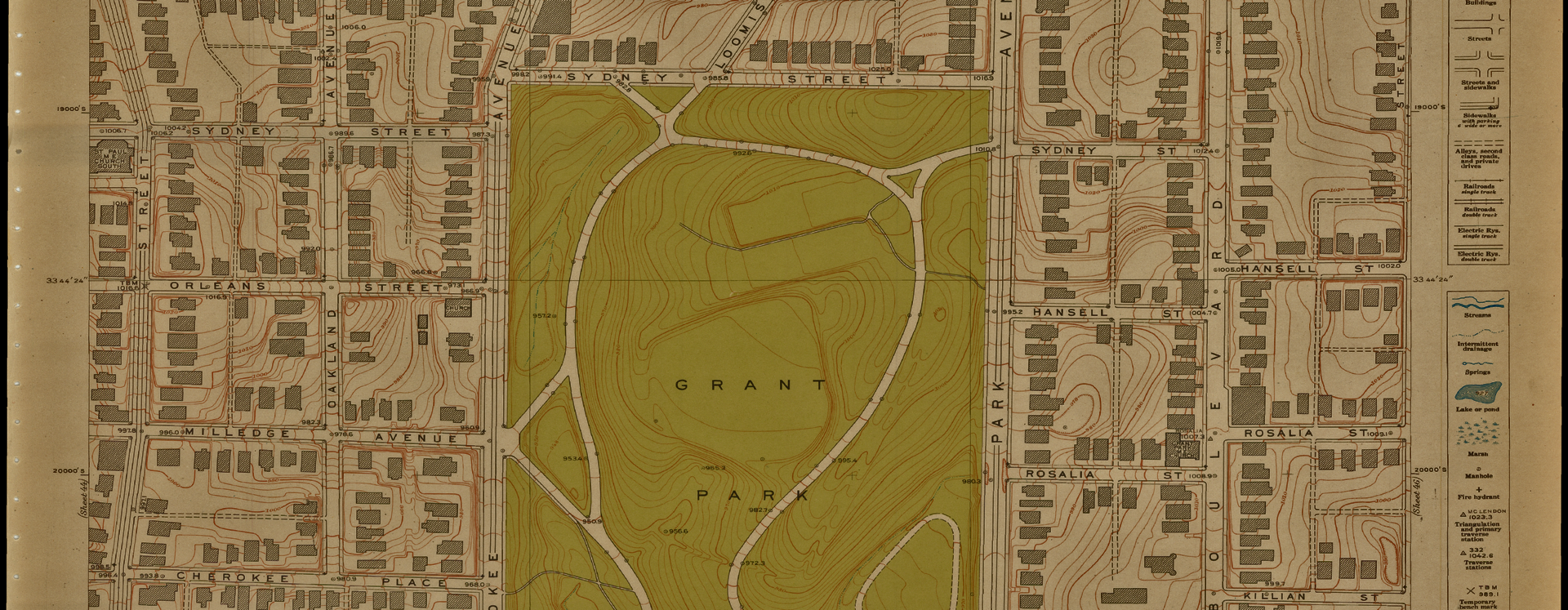
After a good bit of research, lots of trial and error, and working with our colleagues Eric Willoughby at Georgia State University and Amanda Henley at the University of North Carolina, we came up with a process that gave us this:

See the Pen brzJLx by Jay Varner (@jayvarner) on CodePen.

What We Did

We georeferenced our map in the appropriate coordinate system for the map’s area. In our case EPSG:2240. We’ll refer to specific coordinate systems with their EPSG code.

Next we took the resulting GeoTIFF and uploaded it to our GeoServer so the map could be shared via WMS.

Finally, like the examples above, we used Leaflet to display the maps in the browser overlaid on a modern street map.

What We Did Wrong

Our first problem was that the GeoTIFF is a high resolution image. In the first example on this page, we were squeezing a 5,931 x 5,779 pixel image (the full resolution) into a 326 x 276 pixel box (for the zoom level shown above). There’s just too much data to display clearly. Notice that if you zoom all the way in to our original example, the map looks great.

See the Pen OjdGvE by Jay Varner (@jayvarner) on CodePen.

Our other problem was that we used a coordinate system that is inappropriate for web display. Tiled base maps that are provided by organizations like OpenSteetMap are based on EPSG:3857, aka WGS 84 Web Mercator.

GDAL Can Solve those Problems

“GDAL is a translator library for raster and vector geospatial data formats…” This is our three step process.

gdalwarp

We use gdalwarp to reproject, resample, add internal tiling, and compress¹

Reproject

When you georeference a scanned map, you select a projection. For most GIS needs, you will want to use the projection appropriate for the chunk of Earth your map covers. However, for displaying maps on the web, you want to use EPSG:3857².

Resample

gdalwarp offers various algorithms³ for resampling. We suggest you try a few and see what works best. We’ve had good results using average, but many folks will suggest near.

Tiling

GeoTIFFs are organized in 1 pixel strips by default. OpenStreetMap tiles are 256x256. We match OpenStreetMap by adding internal tiles. We’ll go deeper into tiling in our follow up post.

Compress

GeoTIFFs can be huge and it’s not very nice to make users load large files when they don’t have to. GDAL can also compress our GeoTIFFs. There are many compression algorithms, but we’re pretty happy with the results we’re getting with JPEG.

The Command

Here is an example showing how to set all the options. Note the last argument is a path to a file the command will create. Your original GeoTIFF will be preserved.

Syntax

$ gdalwarp -s_srs <source ESPG> -t_srs <target EPSG> -r average -co 'TILED=YES/NO' -co 'BLOCKXSIZE=XXX' -co 'BLOCKYSIZE=XXX' -co 'COMPRESS=ABC' </path/to/source/geo.tif> </path/to/new/geo.tif>

Example

$ gdalwarp -s_srs EPSG:2240 -t_srs EPSG:3857 -r average -co 'TILED=YES' -co 'BLOCKXSIZE=256' -co 'BLOCKYSIZE=256' -co 'COMPRESS=JPEG' atlanta_1928_sheet45.tif processed/atlanta_1928_sheet45.tif

NOTE: We are creating a new copy of the GeoTIFF in a directory called “processed”. You can save it where ever you like.

Now you have a new GeoTIFF projected in Web Mercator and preserved your original.

Add Overviews

We discuss overviews in greater depth in our follow-up post. Remember when we said the main reason the map looked so bad was because there was just too much data? Well, overviews fix that. What happens here is we create internal versions of our image that are smaller and lower resolution.

We also have to tell it to keep our blocks, or internal tiles, at 256, the default is 128. You can set GDAL_TIFF_OVR_BLOCKSIZE as an environment variable, or just override the default with the --config option.

Syntax

$ gdaladdo --config GDAL_TIFF_OVR_BLOCKSIZE XXX -r average </path/to/new.tif> levels (list of numbers)

Example

$ gdaladdo --config GDAL_TIFF_OVR_BLOCKSIZE 256 -r average processed/atlanta_1928_sheet45.tif 2 4 8 16 32

Automation

Obviously if you have more than two maps to process, running these commands on each will get real old real fast. Fortunately, since GDAL is a command line tool, we can automate the whole process. There are wrappers for GDAL in many languages: Python, PHP, .Net, Ruby (though the Ruby gem is no longer maintained and not updated for GDAL 2), etc.

We have automated our process. It’s nice to just run a script and go enjoy some coffee while the computer does all the work.

Conclusion

This has been an evolving process. We found ways to improve the process every time we prepared for a workshop, conference talk, or writing this post. We would love to hear any feedback or suggestions.